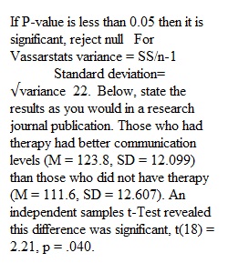
Q Psychology Statistics Dr. Robin Akawi 2022-2023 STATS PACK: Section 4 STATISTICAL ANALYSES – Vassarstats & Excel Worksheets included: Concepts Independent Samples t-Test Excel and Vassarstats Dependent Samples t-Test (a.k.a. repeated measures or correlated samples) Excel and Vassarstats Correlation Excel and Vassarstats One-Way ANOVA for Independent and Repeated Measures samples Vassarstats only for calculations Factorial ANOVA Vassarstats only for calculations Note: All charts and/or graphs should be done in Excel or Google Sheets You will do the following statistics in Excel (or Google Sheets) and Vassarstats. Your goal is to get a consensus amongst the results. You can submit it any time for feedback before the due date, even if not complete. I will leave feedback in the “Comments” section of the “Stats Pack 4” assignment submission link. It will not have a score entered until the end of the semester or once you have completed it and are ready for a grade. INDEPENDENT SAMPLES T-TEST “Effects of Therapy on Communication Levels” 1. We will look at the same scenario, with the variables “Therapy” and “Communication Level” for the two t-Test analyses. The “independent samples t-Test” is first. In this scenario, we randomly assigned spouses to either participate in a new therapy program or to not participate in the therapy program. We need to analyze their communication level scores to see if participating in the therapy program increases “Communication” significantly more than those who do not participate in the program. Use Excel & Vassarstats to run the analyses and fill in the table below: Spouse Therapy Comm Score A Yes 126 B Yes 143 C Yes 126 D Yes 125 E Yes 133 F Yes 109 G Yes 124 H Yes 128 I Yes 99 J Yes 125 K No 118 L No 126 M No 111 N No 116 O No 94 P No 95 Q No 123 R No 105 S No 128 T No 100 CALCULATIONS EXCEL VS Mean communication score YES group Standard Deviation Variance Mean communication score NO group Standard Deviation Variance Degrees of freedom Obtained t score p value Significant or not-significant Reject the null or Fail to reject the null 2. Below, state the results as you would in a research journal publication. 3. Create a bar chart to illustrate the results. ? DEPENDENT SAMPLES T-TEST a.k.a. within-subjects, repeated measures, correlated (not the same as correlation) “Effects of Therapy on Communication Scores Over Time” 4. For this analysis, we want to redo the study but instead of having two groups, we want to investigate the communication levels both before and after participation in the therapy program for all participants. This will control for the extraneous variable of “individual differences” (the two groups we analyzed earlier being different than each other). Therefore, we need to run a “dependent samples t-Test” (because there are “repeated measures” for each participant) and analyze their “before” scores with their “after” scores to see if there is a significant difference in communication for the participants. Here are your data: Spouse Comm Score BEFORE Comm Score AFTER A 115 126 B 135 143 C 116 126 D 115 125 E 129 133 F 99 109 G 113 124 H 119 128 I 88 99 J 117 125 K 110 118 L 118 126 M 102 111 N 115 116 O 83 94 P 87 95 Q 121 123 R 100 105 S 120 128 T 95 100 CALCULATIONS EXCEL VS Mean communication score BEFORE Standard Deviation Variance Mean communication score AFTER Standard Deviation Variance Degrees of freedom Obtained t score p value See note on Excel p-values with “E” Significant or not-significant Reject the null or Fail to reject the null Remember: If Excel shows a p-value with an “E” in it, you will “Extend the decimal to the left however many places that match the number value after the E”. For example, E-07 means extend the decimal 7 places to the left, so 2.437E-07 becomes .0000002437 (WAY less than .0001). ? 5. State the results as you would in a research journal publication. 6. Create a bar chart to illustrate the results. PEARSON CORRELATION Spouse Psych Credits Comm Levels A 3 126 B 15 143 C 6 126 D 3 125 E 6 133 F 6 109 G 9 128 H 6 124 I 3 99 J 6 125 K 3 118 L 9 126 M 3 111 N 3 116 O 1 94 P 3 95 Q 6 123 R 9 105 S 12 128 T 9 100 “The Relationship between Number of Psychology Credits taken and Communication Levels. Consider this, “people who know about people” might influence people’s progress in therapy program? Perhaps, the more psychology credits one takes the higher the success rate in the program. Therefore, we will gather two measures per person (that are interval/ratio data). The first score will be their communication score and the second score will be how many credit hours they have taken in psychology courses. We will then analyze these data with a Pearson correlation (linear correlation). Here are your data: 7. PLOT the data into a “scatterplot” below: 8. Based on what you SEE in the scatterplot, describe the relationship. 9. What is the correlation coefficient for these data? 10. Rather than “significance”, determine the “effect size”. 11. Draw a Venn Diagram to illustrate the overlapping nature of these two variables. ? ONE-WAY ANOVA FOR INDEPENDENT SAMPLES (Note: Vassarstats only) Comm Score BEFORE Comm Score AFTER Comm LONG-TERM 115 126 132 135 143 145 116 126 139 115 125 130 129 133 137 99 109 115 113 124 128 119 128 136 88 99 105 117 125 137 12. Now let’s see if the therapy program has long term effects. We have 30 participants, 10 for each “level” of the IV, which is Time. The time levels are “before” (i.e., no therapy), “after” (immediately after therapy), and “long term” (6 months post treatment). The DV is Communication scores. Complete this ONLY in Vassarstats. Compare/contrast the values and results between the independent samples One-Way ANOVA and the correlated samples One-Way ANOVA. CALCULATIONS Independent Correlated Mean BEFORE Mean AFTER Mean LONG-TERM Standard Deviation BEFORE Standard Deviation AFTER Standard Deviation LONG-TERM Degrees of freedom “between” Degrees of “error” (within) Obtained F ratio p value Significant or not-significant Reject or Fail to reject the null Tukey Post Hoc (a = .05) Independent Correlated M1 vs M2 (before/after) M1 vs M3 (before/long-term) M2 vs M3 (after/long-term) 13. Refer to the Tukey Table above. State your interpretation on the most interesting Post-Hoc Analyses result. Note why. 14. Fill out the remaining values needed in the Source Tables below. ANOVA Independent Source of Variation SS df MS F p-value Between Groups 1259.4667 Within Groups (Error) 4218.4 Total 5477.8669 29 ANOVA Correlated Source of Variation SS df MS F p-value Between Groups 2449.233 Within Groups (Error) 107.2 Ss/Bl 4111.2 9 Total 5477.8667 29 15. Circle/Highlight the values that changed. What was the “MAIN” element that changed? __________ 2x2 FACTORIAL ANOVA (Independent: Therapy x Age Group) (Vassarstats only) NO YES OLDER 9 13 11 10 8 11 9 8 7 10 16 19 14 14 13 19 12 15 13 15 YOUNGER 11 15 10 16 16 16 12 11 14 15 13 17 15 18 17 16 18 15 18 16 In this last analysis, we are investigating communication scores for both older and younger individuals who either went through communication therapy or did not. Thus, our analysis is a 2x2 Factorial ANOVA for independent samples. 16. Create a MEANS TABLE for our data. 17. Generate a LINE GRAPH based on the four group means in the table above. 18. Fill out the remaining values needed in the Source Table below: ANOVA for Effects of Age and Therapy on Communication Scores Source of Variation SS df MS F P-value Age Group (Rows) 70.23 Therapy (Columns) 164.02 Age Group x Therapy (R x C) 18.23 Within Groups (Error Variability) 154.9 Total 407.38 39 19. INTERPRETATION (How would you explain these results to others?): 20. Paste screenshots of your output from Excel (or Google Sheets) and Vassarstats below that are not showing elsewhere in this packet.
View Related Questions